From Bayes To MCMC - Sampling Techniques

This post describes probabilistic fundamentals in sampling techniques. It is very useful in taking samples with non-analytical form distribution. It is assumed that you already know Bayesian theory, or at least heard about it. Bayesian theory is firstly introduced and then followed by the functional description of MCMC without mathematical equations.

Bayes Inference

In SLAM and state machine:

\[P(X|Z) = \frac{P(Z|X)P(X)}{P(Z)} = \frac{P(Z|X)P(X)}{\sum_{i}P(Z|x_i)P(x_i)} \\ \Rightarrow \underbrace{P(X|Z)}_{\text{Posterior}} \propto \underbrace{P(Z|X)}_{\text{Likelihood}} \underbrace{P(X)}_{\text{Prior}}\]

Where $Z$ is the observation or input feature, the set of all possible observation which forms the observation space or feature space. If you take a sample from $Z$, this sample shall denoted as $z$.

$X$ can be seen as state in state machine or the model in machine learning to prediction with hidden internal parameters, which forms the prediction space.

What Bayes Inference describes is a inverse of Cause and Effect Theorem. $X$ is the cause which can be abstract and hard to be explained(especially in the context of machine learning), such as being a woman, or a robot pose, and corresponding $Z$ may be the lang hair or environment of the robot.

Likelihood describes the probability(sometimes also called model) that a woman might have lang hair and robot which might be in the specific space(with little uncertainty) observing a environment setting. It can also be interpreted as because …, … such as because she is a woman, there is a high probability she has lang hair; because the robot is in a special pose, there is a high probability that it observes the universe in a special specific fixed viewpoint. As the probabilistic theory has a property of being stochastic, you can try not think universe deterministic, this may gives you a easy to understand why probabilistic theory is so important.

Posterior switched the the condition and variable compared to Likelihood, and it describes how probably that a lang hair person is a woman, and how probably a robot is in the special pose, given its observation. Posterior is important because it gives a way to describe analyse model or state with observation, and the observation is relatively easy to be obtained. However the way it works is still not generally accepted.

Bayesian credible intervals can be quite different from frequentist confidence intervals for two reasons:wiki

• credible intervals incorporate problem-specific contextual information from the prior distribution whereas confidence intervals are based only on the data;
• credible intervals and confidence intervals treat nuisance parameters in radically different ways.

Prior is the trouble maker, because a priori distribution is your subjective judgment about the probability distribution of a parameter before you obtain experimental observations. subjective judgment is the reason why Bayesian statistics are not well recognized, and science prefer objective. However it is actually very useful.

An Example

You might still feel confused about Bayes Inference, Lets have a simple example to explain Prior and Likelihood:

Suppose you are producing something, and there are 2 procedures to produce posterior, the likelihood and prior distribution are both gaussian distribution(this is made on purpose to form a conjugate prior so that posterior is also a gaussian):

\[\underbrace{P(X|Z)}_{\substack{Posterior}} \propto \underbrace{P(Z|X)}_{\substack{Likelihood}} \underbrace{P(X)}_{\substack{Prior}} = N(z|\mu, \sigma^2) \cdot N(\mu|\mu_0, \sigma_0^2)\]

What prior samples is the $\mu$ and $\mu$ is the parameter for sampling $x$, in other words, with different sampled $\mu$, the likelihood can be very different! as the result, Posterior vaires with the prior distribution. This is the key why Prior is the trouble maker, This is why the mathmatikers are trying so hard to find a way to determine prior.

In the sampling of Prior distribution(process of production), the “real” feature/state $x^*$($\mu$) is a sample, which should be subject to Prior distribution $N(\mu | \mu_0, \sigma_0^2)$.

In the sampling of likelihood distribution(process of measurement), $\hat{z}$ is the measurement and is subject to $N(z|\mu, \sigma^2)$. In the following figure, $\mu = 102$ and observation has $\sigma = 3$.

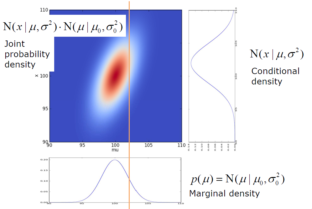
Fig. Visualization of joint probability distribution(notation difference: $x$ in the figure correspond to measurement), source: Claus Brenner

Now you can easily find that what posterior is for, posterior is more interested in the $X$ with observation $Z$, in the example, it means how does our knowledge about $\mu$ changes after a measurement, corresponding to “horizontal” conditional density. In the following figure, measurement $x = 97$

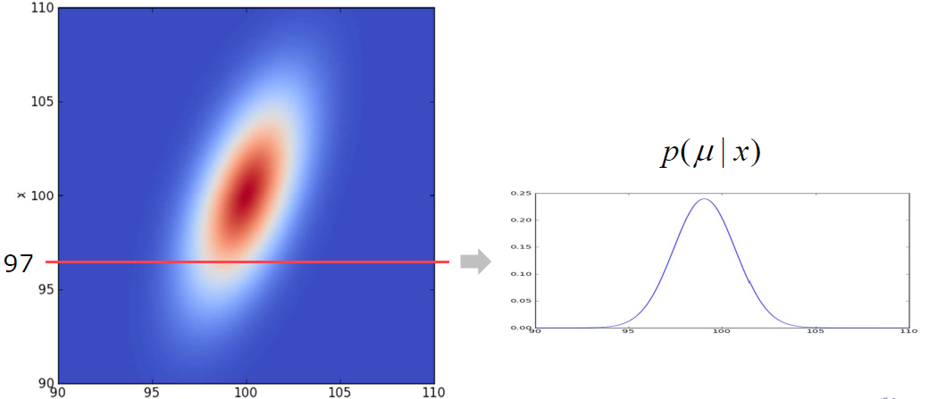
Fig. Visualization of posterior distribution(notation difference: $x$ in the figure correspond to measurement), source: Claus Brenner

In above case, P(\mu|x) = $N(\mu|\mu_{post}, \sigma_{post}^2)$ with $\mu_{post} = 99.0769$ and $\sigma_{post} = 1.66410$

General Case

Analytical from is not always the available, gaussian in the example is a special case. Generally we are interested in certain quantities such as expectation of a function with variable in the probability distribution or Maximum a posteriori (MAP) estimation, However, because of unknown prior density of $p(x)$, it is usually approximated by

\[E[f] = \int f(x)p(x)dx\] \[E[\hat{f}] \approx \frac{1}{m} \sum_{j=1}^{m}f(x_{j}) \text{ with } x_j \sim p(x)\] \[Var[\hat{f}] \approx \frac{1}{m} E[(f - E[f])^2]\]

Task Definition and Methods

Thus, the task is sampling from a (complex) distribution, this is exactly why MCMC is included in this post. We need a random sample generator for a random variable with density p(x)

Inversion Trick

Suppose you already know CDF and PDF, inversion trick is realized by the inverse function to transfer the known distribution to unknown CDF.

Suppose $U \sim Uniform(0,1)$ and $V:= F^{-1}(U)$, then it follows:

\[F(v) = P(V \leq x) = P(F^{-1}(U) \leq x) = P(U \leq F(x)) = F(x)\]

So, to sample $x \sim f(x)$ we can draw $U \sim Uniform(0,1)$ and then compute $x = F^{-1}(U)$

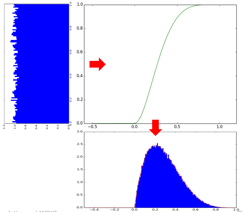
Fig. Inverse trick example, source: Claus Brenner

Limitation:

• $x = F^{-1}(U)$ has to be able to be computed, you can try a multiple mode gaussian distribution to find out whether it is okay.
• not suitable for distributions which are not given in a usable form or for which an inverse CDF cannot be computed or cannot be computed efficiently.

Accept-Reject Method

We want to sample from $p(x)$, as we don’t know the form of $p(x)$, we add another dimension for sampling namely $U$, with $U$ aligned to probabilistic space of $p(x)$, then:

\[X \sim p(x) \iff (X,U) \sim Uniform \{(x,u) | 0<u<p(x) \}\]

The sampling process in $X \in [a,b]$ with unknown p(x) is converted to uniform sampling from $X \in [a,b]$ with and $U \in [0,1]$. Counting accepted samples to $X$ space can reproduce the $p(x)$, and the acceptance criterion is $0<u<p(x)$.

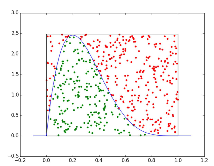
Fig. Accept Reject example, red dots is rejected and green are accepted, source: Claus Brenner

Limitation:

• Efficiency depends on the probability of acceptance(comparison on area size), to improve the efficiency you may replace the extra uniform distribution of $U$ to other distributions such as gaussian, but it has to enclose the area of $p(x)$, what has to be mentioned is that sampling on $U$ has to be uniform, because you want to accumulate the samples in this dimension.

• For log-concave functions, the algorithm can be extended so that the instrumental density is iteratively adjusted and adapted to the density of f. (See Robert & Casella.)

• Distributions with high dimensionality is hard to find a proper density function $q(x)$.

Importance Sampling

This method is used for —computing expected value, however, drawing samples subjected to $p(x)$ cannot be achieved easily.

\[E[f] = \int f(x)p(x)dx = \int f(x)\frac{p(x)}{q(x)} q(x) dx \\ = \int \underbrace{f(x)\frac{p(x)}{q(x)}}_{\text{Approximation Function}} \underbrace{q(x)}_{\text{Instrumental Density}} dx\]

Then the calculation can be approximated:

\[E[\hat{f}] \approx \frac{1}{m} \sum_{j=1}^{m}f(x_{j})\underbrace{\frac{p(x_j)}{q(x_j)}}_{\text{Weight/Importance}} \text{ with } x_j \sim q(x)\]

As an instrumental density, you know the analytical form of $q(x)$ and you can take samples from it. On the other hand, you have $p(x)$ in unknown form, but given lots of samples of $x$, you can approximate $p(x_j)$

Limitation:

• the choice of $ q(x) $ influences the convergence properties

Gradient ascent(only MAP)

This method is used for computing local maxima, however, drawing samples subjected to $p(x)$ cannot be achieved easily.

• Start with an arbitrary camera location
• Evaluate the target function
• Propose a random step (random length and direction)
• Evaluate the target function there as well
• Accept if the value increases.

This is the most normal way, and shall not be introduced.

Limitation:

• Only local maxima can be achieved.

MCMC(Markov Chain Monte Carlo)

What is MCMC

As we can see from the name, MCMC consists of two MCs, namely Monte Carlo Simulation (MC) and Markov Chain (also referred to as MC). To understand the principle of MCMC we must first figure out the principle of Monte Carlo method and Markov chain. The MCMC method is used to estimate the posterior distribution of the parameter of interest by random sampling in probability space.

Monte Carlo

Monte Carlo is the method to approximate the value with simulation, for example you want the the value of $\pi$, and you can take samples from a square and count samples in the circle. As introduced in the above section, directly sampling from p(x) can be hard, $\theta$ is our target value, such as expectation. Following the the normal format of Monte Carlo with Importance sampling:

\[\theta = \int_a^b f(x)dx = \int_a^b \frac{f(x)}{p(x)}p(x)dx \approx \frac{1}{n}\sum\limits_{i=0}^{n-1}\frac{f(x_i)}{p(x_i)}\]

Markov Chain

Markov property:

\[P(X_{t+1} |...X_{t-2}, X_{t-1}, X_{t} ) = P(X_{t+1} | X_{t})\]

Following is a markov chain with transition matrix:

\[T=\left( \begin{array}{ccc} 0.9&0.075&0.025 \\ 0.15&0.8& 0.05 \\ 0.25&0.25&0.5 \end{array} \right)\]

Fig. Markov Chain Model, source: Wiki

Set a random node as a start denoted as $X_1$, and after a while of transition until $X_n$, you can find that $\lim_{n \to \infty}P_{ij}^n$ in each colom remains the same.

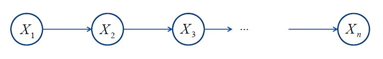
Fig. Random Walking Process, source: Wiki

\[T=\left( \begin{array}{ccc} 0.625&0.3125&0.0625 \\ 0.625&0.3125&0.0625 \\ 0.625&0.3125&0.0625 \end{array} \right)\]

MCMC usually samples from stationary distribution, and sampling algorithms is listed below but not put in scope in this post.

Metropolis-Hastings

Please refer link

Gibbs

Please refer link

reversible jump MCMC

Please refer link