Fundamentals In Deep Learning

In this post, the basic knowledge of deep learning involving classification and regression shall be explained. Firstly, the working mechanism and mathematical abstraction of neural networks and procedures to train a network. Secondly, the detection task and segmentation task based on CNN, including essential breakthroughs such as ResNet and FCN. Third, basic principles on object detection are introduced.

Mathematical Abstraction

Deep learning is a branch of machine learning applied to solve complex NP-hard problems by neural network methods. In abstraction, deep learning models have a decent formulation as follows:

Suppose a target space $Y$ is given, which ought to be approximated by a function $F$ with features $X$ as vairable and $P$ as internal parameter (if necessary), which is formalized as: \begin{equation} F(X|P) \mapsto Y \end{equation} According to the continuity of $Y$, model $F$ can be divided into two branches:

• Classification: Prediction on the discrete label. A classification algorithm may predict a continuous value, but the continuous value is in the form of a probability for a class label.

• Regression: Prediction on continuous quantity. A regression algorithm may predict a discrete value, but the discrete value in the form of an integer quantity.

Most deep learning methods works in a supervised manner, which needs data to learn from “experiences”. LossLearning is targeted by loss calculation, then the judgment based on learned experience can be accurate. This process to learn from experience/samples is called training, which optimizes the model recursively by approximate target function $F$ by learning from examples. High-dimensional(reason for NP-hardness) features of the training sample are fed to the deep learning model. The model approximates itself under the instruction of the loss function, which is hardly interpretable but actually works; thus, deep learning models are often called a black box.

Multiple layer Perceptron

Perceptron: a basic unit of deep learning model	Multi Layer Perceptron: a combination of perceptrons

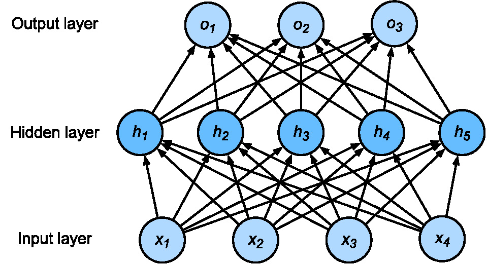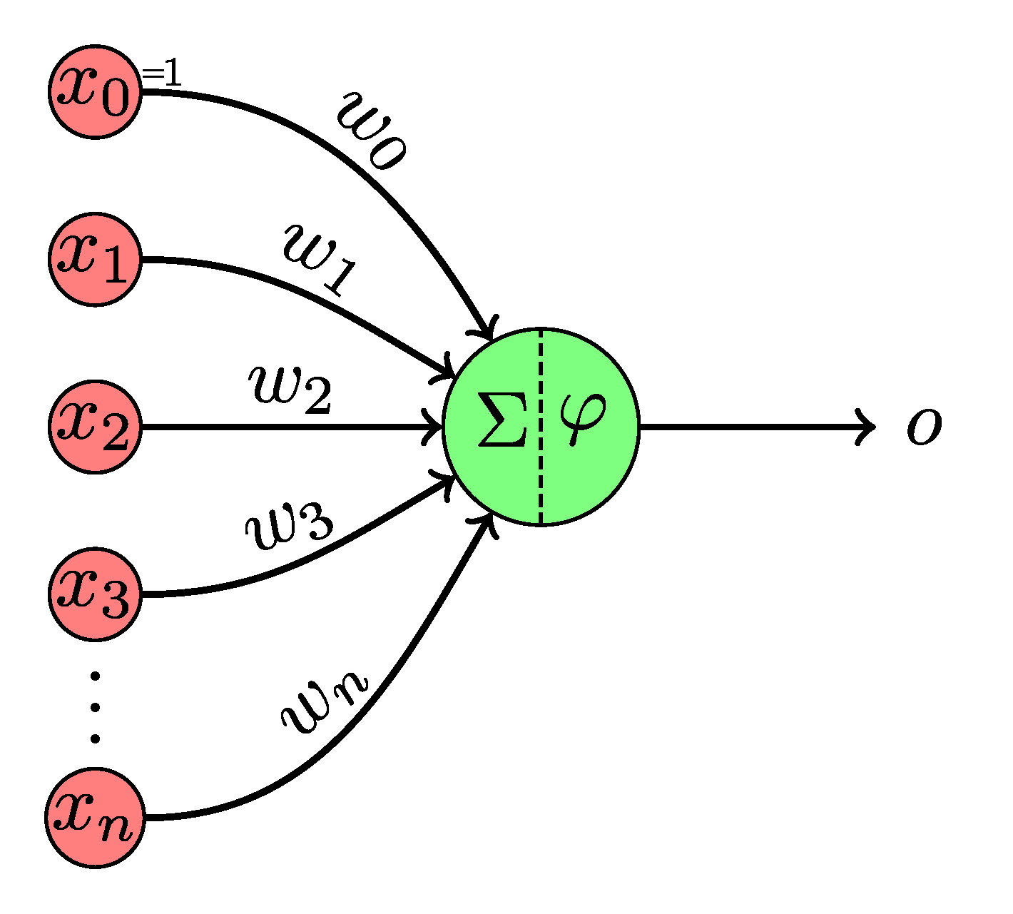
Fig. 1 perception and multi layer perceptron: abstraction of deep learning units (source: wikipedia, link)

Parameters	Description
$x_1,\dots,x_n$	Input Vector
$w_1,\dots,w_n$	Weights
$\phi$	Activation Function
$w_0$	Bias

The basic computation unit in a neural network is called perceptron, which is abstracted to a linear combination of inputs(features) with weights and bias followed by an activation function shown in Fig.1. Each perceptron has its associated internal parameters $P$ weight and bias, which shall be learned/tuned during training. Weights assigned to the input feature models the importance of each input channel. Bias models a shift to the overall input. Activation function forms a nonlinear transformation from the weighted arithmetic of features, such as sigmoid function and ReLU. Without the activation function, the neuron network shall be a complex combination of many linear combinations, which is still linear. Therefore, activation functions are necessary to enable networks to have the ability to simulate nonlinear functions.

Perceptron can be mathematically expressed as: \begin{equation} y = f_{act}(\sum_{i=1}^{n} x_i w_i + b) = f_{perceptron}(x_1, \dots, x_n | w_1, \dots, w_n, b ) \end{equation} where:

Paramters	Description
$w_i$	weights, internal parameters of model
$b$	bias, internal parameter, also interpreted as $w_0$
$x_i$	features, input
$f_{act}$	activation function
$f_{perceptron}$	model function

Training & Inference

Training is the process of adjusting weights and bias $P$ to get the proper values so that the features $X$ feed into neural networks output the right prediction that is desired to be consistent with the ground truth. Because of the problems that neural networks solve are usually NP-hard, and there are no closing solutions to weights and bias, we usually take optimization techniques to find a “proper” solution. However, it is usually not a perfect solution. Training means exactly optimization in deep learning, but there are many practical techniques.

The loss/objective/cost/error function is formalized to measure the difference between ground-truth/desired output $Y^*$ and predicted output $Y$ in the optimization aspect. The loss function is usually optimized by stochastic gradient descent(SGD) or mini-batch gradient descent. Gradient descent points out the direction to move, “Stochastic” means apply gradient descent on only one stochastically sample from the training data $X$ and “mini-batch” for a subset of training samples $X$.

The inference is a process to make predictions with the trained parameters $P$, in contrast to training. The internal parameters $P$ are the model variables to be solved. Inference takes the internal parameters $P$ as fixed parameters to output a prediction $Y$ with a given input $X$ as a variable.

Loss

As mentioned above, the loss function measured the difference between the model’s output and desired output, which indicates the loss function often needs to be customized to suit task requirements. Such as focal loss, IOU loss family(link link link) in the object detection task. Although well-designed loss function makes specific models more effective during training, many basic loss functions are still fundamentally beneficial. Researchers prefer a loss function where the space of “proper” weights maps onto a smooth (but high-dimensional) landscape that the optimizer can reasonably navigate via iterative updates to the model weights.

Loss functions are also divided into classification and regression loss according to specific tasks, for example, binary multi-class entropy loss for classification. \(\begin{equation} Entropy = s-\sum_{c=1}^My_{o,c}\log(p_{o,c}) \end{equation}\) where

Parameters	Description
$M$	number of classes (dog, cat, fish)
$Log$	Natural Log
$y$	1 if prediction ${c}$ matches observation ${o}$, else 0
$p$	predicted probability observation o is of class ${c}$

Mean absolute error(MAE), L1 loss: \(\begin{equation} S = \dfrac{\sum_{i=0}^n|y_i - h(x_i)|}{n} \end{equation}\) Mean square error(MSE), L2 loss:

\(\begin{equation} S = \dfrac{\sum_{i=0}^n(y_i - h(x_i))^2}{n} \end{equation}\) where

Parameters	Description
$x_i$	features
$h$	model function
$y_i$	ground truth of predictions
$n$	batch-size

L2 loss has a fast convergence, but the L1 loss is more robust to outliers. L2 loss tends to give the mean target value, while L1 is the median value, and mathematically the median is robust than the mean value considering non gaussian distribution. MAE always has the same gradient in each direction at negative infinity and positive infinity. It would slow down at the stochastic gradient descent process, making it fluctuate when it is close to the origin. There are some other losses such as Huber Loss, Hinge Loss but not included here.

Backpropagation

Backpropagation is a significant breakthrough in deep learning history, and it enables gradient descent on all the parameters in the complex multiple-layer model by the chain rule.

Suppose an activation function ${f^L}$ in a neural network is given. Forward propagation for simple MLP can be described as follows:

\begin{equation} { g(x):=f^{L}(W^{L}f^{L-1}(W^{L-1}\cdots f^{1}(W^{1}x)\cdots ))} \end{equation} where

Parameters	Description
$g(x)$	model function
$f^L$	activation function at layer $L$
$W^L$	weights and bias of layer $L$ with bias represented as $w_0$

And the cost function is formalized as: \begin{equation} \min_{W} Cost(y,g(x)) = \min_{W} Cost(y,f^{L}(W^{L}f^{L-1}(W^{L-1}\cdots f^{2}(W^{2}f^{1}(W^{1}x))\cdots ))) \end{equation}

Denote the weighted input of each layer as $z^{l}$ and the output of layer ${l}$ as the activation ${\displaystyle a^{l}}$. For backpropagation, the activation ${\displaystyle a^{l}}$ as well as the derivatives ${\displaystyle (f^{l})’}$ (evaluated at ${\displaystyle z^{l}}$) must be cached for use during the backwards pass. Then the chain rule can be applied to calculate the derivatives of loss in terms of the inputs: \begin{equation} {\displaystyle {\frac {\partial Cost}{\partial a^{L}}}\cdot {\frac {\partial a^{L}}{\partial z^{L}}}\cdot {\frac {\partial z^{L}}{\partial a^{L-1}}}\cdot {\frac {\partial a^{L-1}}{\partial z^{L-1}}}\cdot {\frac {\partial z^{L-1}}{\partial a^{L-2}}}\cdots {\frac {\partial a^{1}}{\partial z^{1}}}\cdot {\frac {\partial z^{1}}{\partial x}}.} \end{equation}

Optimizer

In standard optimization methods, there are also other methods such as Gauss-Newton and Levenberg-Marquardt. They are still not widely used in machine learning, especially in deep learning, because it is hard to calculate the second derivative, and its operation first derivative is too complex. In the community of deep learning, SGD and other developed optimizers such as (SGD, SGDM, AdaGrad, AdaDelta, Adam) and are generally accepted. A framework of SGD based optimizer is introduced in following alogrithm:

SGD takes no advantage of momentum: \begin{equation}\label{eq:sgd} m_t = g_t; V_t = I^2 \end{equation} However, SGD has a slow convergence and tends to oscillate across the narrow ravine. The negative gradient will point down one of the steep sides rather than along the ravine towards the optimum, which brings the momentum. \begin{equation}\label{eq:momment} m_t = \beta_1 m_{t-1} + (1-\beta_1)g_t; V_t = I^2 \end{equation} Momentum makes the convergence faster with inertia to keep the speed of the previous gradient update.

Deep Neural Networks

Vanilla neural networks with few layers cannot solve complex problems, whereas models with too complex layers(many fully connected layers) tend to overfit data and lead to hard training. Meanwhile, as the network deepens, problems such as vanishing gradients and gradient explosion make researcher hard to train the desired model. Most importantly, what happened in the network is a black box in training. Even now, this problem is not solved yet. Many researchers design the network and experiment to see its performance iteratively to push the research frontier.

In the competition of ImageNet in 2011, a deep learning model attracted enormous attentions. Since then deep learning method has been a hotter topic compared with other machine learning techniques in AI science. Here are CNN and FCN introduced to give the readers a scope of “deep” sense.

Convolutional Neural Network(CNN)

CNN is similar to filter techniques in image processing. but CNN takes trainable filters and applies them multiple times(deeper) in a sequence. Because filters take a sliding window manner to process images, CNN are borned with advantages of feature alignment which is interpreted as spatial-invariant/translation-invariant properties, spatial-invariance is significant in tasks like semantic segmentation. Besides, CNN warp features in the neighborhood, making the learning of local interactions/relations in a perceptive field possible.

Besides, CNN has a property to avoid overfitting due to shared weights, which also significantly reduced the number of parameters compared with FCN. The amount and size of convolution kernel can also be maintained to fit the task requirements for training. It is generally acknowledged in deep learning community that low-level features are convolved to form high-level features as the network deepens.

CNN often collaborates with other layers such as the pooling layer(max pooling, average pooling) and normalization layer to avoid overfitting and gradient vanishing problems. Max Pooling layers select the response of neurons in a local neighborhood(in a hard way compared with soft in “softmax”) and reduce the resolution, meanwhile the perceptive fields are enlarged, more features are fused or important features are selected, whereas spatial resolution is lost. Normalization layers(Batch Norm, Weight Norm, Layer Norm, Instance Norm, Group Norm, Batch-Instance Norm, Switchable Norm) maintain the distribution of neuron responses, ensuring that after multiple layers, the response from one path is not dominant(explode).

CNN has now developed to be a backbone in object detection, which can be seen as a feature pool to support subtasks such as detection and segmentation. A backbone with rich representative features directly affects the performance of the model.

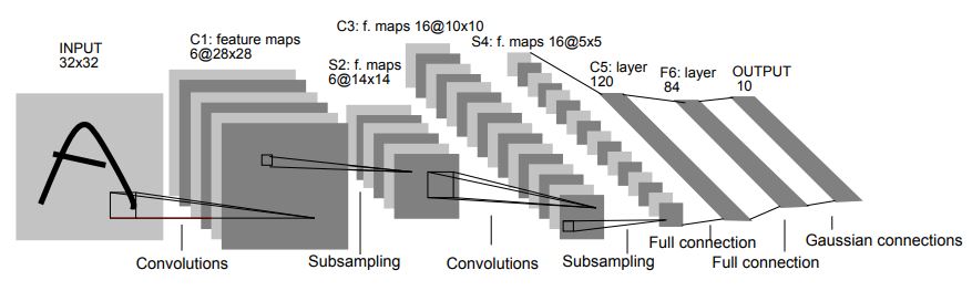
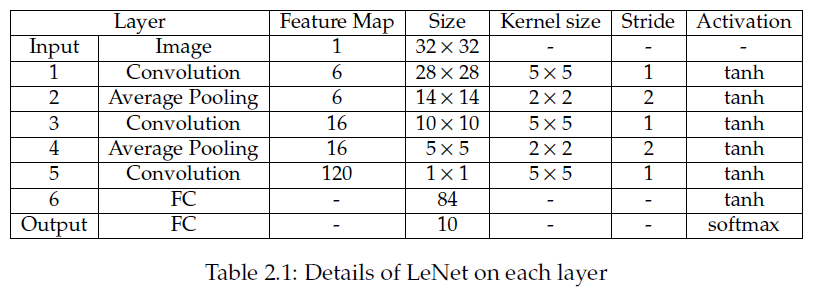
As shown in following image, LeNet-5 is an example for CNN.

Fully Convolutional Network(FCN)

For semantic segmentation, CNNs are used to fuse/encode features then FCN are used to separate/decode features into semantic classes(called deconvolution) and make predictions more comparable with ground truth labels directly.

Max Pooling layers and convolutional layer with stride over 1 reduces the resolution of feature maps by selecting the strongest impulse or average responses from the front layer (downsampling), but spatial consistency is lost in local receptive field in this process. Although upsampling layers(transpose convolution) take features from low resolution to high resolution, spatial information is still hard to be reproduced. The trick that researchers apply is skip connection for featrure map with same resolution. Since shallower layers have more accurate spatial consistences because of less pooling operations, element-wise addition/contanentation between shallower layers, and upsampling layers fuses spatial invariance information and semantic features the outputs could be consistent with the input size.

Following this idea, FCN made a milestone in the development of semantic segmentation. FCN is completely composed by convolution which means the requirement for size of the input images is eliminated.